

10 Python one-liners for generating time series features
introduction
Time series data Building effective and insightful predictive models typically requires deep understanding. Two important properties are important in time series forecasting: Expression and granularity.
- Representation involves transforming raw temporal data (such as daily or hourly measurements) into useful patterns using meaningful approaches.
- Granularity is the analysis of how accurately such patterns capture change over time.
The difference is subtle, as they are two sides of the same coin, but one thing is for sure: both are achieved in the following ways. feature engineering.
This article introduces 10 simple Python one-liners for generating time series features based on various underlying characteristics and properties of raw time series data. These one-liners can be used alone or in combination to help create more informative datasets that reveal more about the temporal behavior of your data: how it evolves, how it fluctuates, and what trends it shows over time.
In this example, panda and Numpy.
1. Lag function (autoregressive expression)
The idea behind using autoregressive representations or lag features is simpler than you might think. That is, it consists of adding the previous observation to the current observation as a new predictor feature. Essentially, this is probably the simplest way to express temporal dependencies, such as between the current time and the previous time.
As the first one-liner sample code in this list of 10, let’s take a closer look at this one.
This one-liner example uses a raw time series dataset as DataFrame called dfthe name of one of the existing attributes is 'value'. Note the argument. shift() You can adjust the function to get the registered value n Time or observation before the current time:
|
D.F.(‘lag_1’) = D.F.(‘value’).shift(1) |
For daily time series data, if you want to get the value before a particular day of the week (e.g. Monday), it makes sense to use: shift(7).
2. Rolling average (short-term smoothing)
To capture local trends or smoother short-term fluctuations in the data, it is usually useful to use rolling measures across the data. n Past observations leading to current observations: This is a simple but very useful way to smooth out sometimes chaotic raw time series values on a particular feature.
This example creates a new feature for each observation that contains the moving average of the three previous values of this feature in recent observations.
|
D.F.(“Rolling average_3”) = D.F.(‘value’).rolling(3).average() |
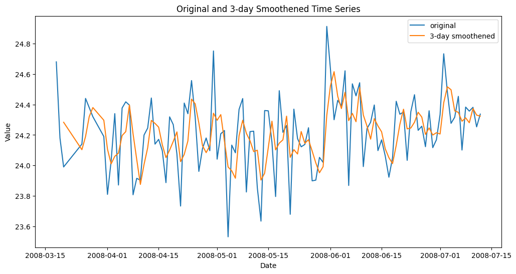
Smoothed time series features using moving average
3. Rolling standard deviation (local volatility)
Similar to rolling averages, there is also the possibility of creating new features based on rolling standard deviations, which are effective for modeling how much successive observations vary.
This example introduces the ability to model the variation of recent values over a moving window of one week, assuming daily observations.
|
D.F.(“Rolling_std_7”) = D.F.(‘value’).rolling(7).standard() |
4. Extended average (cumulative memory)
Extended averaging calculates the average of all data points up to and including the current observation in the time series. So it’s like a rolling average where the window size is always increasing. It is useful to analyze how the average value of a time-series attribute changes over time to better identify long-term upward or downward trends.
|
D.F.(‘expanding_mean’) = D.F.(‘value’).expand().average() |
5. Differentiation (trend removal)
This technique is used to remove long-term trends and emphasize rates of change. In non-stationary time series, it is important to stabilize the rate of change. Computes the difference between consecutive observations (current and previous) of a target attribute.
|
D.F.(“Difference_1”) = D.F.(‘value’).difference() |
6. Time-based features (extraction of time components)
Simple, but very useful in real-world applications, this one-liner allows you to deconstruct and extract relevant information from a complete date/time feature, or create indexes around time series.
|
D.F.(‘month’), D.F.(“day of week”) = D.F.(‘date’).dt.month, D.F.(‘date’).dt.day of week |
Important: Carefully check whether the time series’ date and time information is included in a regular attribute or as an index in a data structure. If it’s an index, you may need to use this instead.
|
D.F.(‘time’), D.F.(“day of week”) = D.F..index.time, D.F..index.day of week |
7. Rolling correlation (temporal relationship)
This approach takes rolling statistics over time windows one step further and measures how recent values correlate with lagged values, thereby helping to discover evolving autocorrelation. This is useful, for example, to detect regime shifts, which are sudden and sustained behavioral changes in the data over time that occur when rolling correlations begin to weaken or reverse at some point.
|
D.F.(‘Rolling Col’) = D.F.(‘value’).rolling(30).wrong(D.F.(‘value’).shift(1)) |
8. Fourier features (seasonality)
Sine Fourier transforms can be used on raw time series attributes to capture periodic or seasonal patterns. For example, applying a sine (or cosine) function transforms the periodic day-of-week information underlying date and time features into continuous features that are useful for learning and modeling annual patterns.
|
D.F.(‘Fourier_Shin’) = NP.sin(2 * NP.P* D.F.(‘date’).dt.day of the year / 365) D.F.(‘Fourier_Cos’) = NP.costume(2 * NP.P* D.F.(‘date’).dt.day of the year / 365) |
This example uses a 2-liner instead of a 1-liner for a reason. Using both sine and cosine together is better for capturing the overall picture of possible cyclical seasonal patterns.
9. Exponentially weighted averaging (adaptive smoothing)
Exponentially weighted averaging (EWM for short) is applied to obtain exponentially decaying weights that increase the importance of recent data observations while preserving long-term memory. This is a more adaptive and somewhat “smarter” approach that prioritizes recent observations over the distant past.
|
D.F.(‘ewm_mean’) = D.F.(‘value’).Hmm(span=5).average() |
10. Rolling entropy (information complexity)
For the last part, let’s do some more math. The rolling entropy of a particular feature over a time window calculates how random or distributed the values are over that time window, thereby revealing the amount and complexity of information within it. Lower values of the resulting rolling entropy indicate a sense of order and predictability, whereas higher values of these indicate more “chaos and uncertainty.”
|
D.F.(‘rolling_entropy’) = D.F.(‘value’).rolling(10).apply(lambda ×: –NP.sum((p:=NP.histogram(×, trash can=5)(0)/Ren(×))*NP.log(p+1e–9))) |
summary
In this article, we reviewed and illustrated 10 strategies (each spanning one line of code) for extracting various patterns and information from raw time series data, from simple trends to more advanced trends such as seasonality and information complexity.